Utilities
Track Visualization
To check the tracking results visually, the PyForTraCC library provides a visualization module. This module enables you to view
the tracking results based on data in the tracking table. Before calling the plot and plot_animation functions, make sure
to add geospatial information to the name_list configuration.
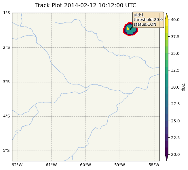
Example: Static Plot
The following code generates a static plot of the tracked rain cells at a specific timestamp.
pyfortracc.plot(timestamp='2014-02-12 10:12:00', name_list=name_list, read_function=read_function,
                cbar_title='dBZ', info=True, grid_deg=None)
Example: Animated Plot
To create an animated visualization of the tracking data, use the plot_animation function. This function generates a sequence
of plots over a specified time range, allowing you to observe changes in the tracked rain cells over time.
pyfortracc.plot_animation(read_function=read_function, name_list=name_list,
                            figsize=(14,5), cbar_title='dBZ',
                            threshold_list=[20], grid_deg=None,
                            info=True, info_col_name=True,
                            start_stamp='2014-02-12 10:00:00',
                            end_stamp='2014-02-12 14:12:00')
Spatial Conversion
The library includes a spatial_conversions utility that enables conversion of data from the tracking_table to popular geospatial formats such as NetCDF, TIFF, Shapefiles, and GeoJSON. To use this module, additional spatial information must be added to the name_list, including grid size and geospatial coordinates.
These utility functions enhance the usability of PyForTraCC by facilitating both data visualization and data format compatibility with other geospatial tools.